Sunday, August 29, 2010

Entropy, volume and temperature


This screencast shows a Molecular Workbench simulation I made to illustrate the connection between entropy, volume, and temperature.


Each simulation runs for 50 picoseconds (ps) and records how much time the two particles spend together (as a dimer) and apart (as monomers).  These times are a reflection of the relative probabilities of the dimer (pdimer) and monomers (pmonomers).
In the first simulation of the screencast the particles spend 38.3 ps together and 11.7 ps apart.  When I double the volume (while keeping the temperature constant) in the second simulation, the particles spend 32.7 ps together and 17.3 ps apart.


This makes intuitive sense: when the particles are not together they have a harder time finding each other again in a bigger volume.  Put another way, the probability is lower that the particles find each other when they move in a larger volume.


Now I want to connect this intuitive explanation with a thermodynamic one (i.e. an explanation in terms of free energy and entropy) :


The relative probability of being together and apart is given by the change in free energy (ΔA) on going from the dimer to the two monomers (dimer -> 2 monomers)
The increase in pmonomers/pdimer (from 0.31 to 0.53) on doubling the volume must mean that ΔA  decreases when the volume is doubled.  Statistical mechanics tells us that the only thermodynamic term in A that is affected by volume (V) is the translational entropy
 and that an increase in volume will increase the entropy of a particle
So when the volume is doubled the entropy of each particle (the dimer and each monomer) is increased by Rln(2). As a result ΔS for the reaction dimer -> 2 monomers increases [by Rln(2)] and ΔA = ΔU - TΔS decreases by RTln(2).  So the probability of the dimer relative to the monomers decrease because the entropy is increased when the volume increases.


In the last simulation of the screencast I double the temperature (while keeping the volume constant) compared to the first simulation. As a result the particles now spend less time together (19.2 ps) than apart (30.8 ps).

This also makes intuitive sense: the dimer is more likely to be struck by a particle with a kinetic energy larger than the potential energy that is holding it together: Furthermore, when the monomers happen to collide they are more likely to have a combined kinetic that is larger than the potential energy holding the dimer together, i.e. "with too much kinetic energy to stick together".

As before, this must mean that ΔA decreases when the temperature is increased.  The increase in translational entropy due to temperature is indeed larger than for the volume
and consistent with the observed larger change in the time the particles spend apart.

If you think of the dimer as a crude model of a salt you want to dissolve, this explains why dilution (increasing the volume) or heating increases the solubility (the amount you can dissolve).  Conversely, increasing the concentration (the amount of particles per volume) or decreasing the temperature helps dimer formation and, in a larger sense, self assembly.

You can play around with it on this web page, or you can download the model if you have Molecular Workbench installed on your computer. Enjoy!

Clarifications and approximations
 You may wonder why I discuss the Helmholtz free energy change (ΔA; some books use ΔF) rather than the Gibbs free energy change, when the volume changes.  This is because the volume of the system (i.e. the two compartments) does not change. Another argument is that no work is done during the expansion.

I have implicitly invoked the ergodic hypothesis which states that the probability computed using a collection of molecules at a single instant in time is equal to the probability computed for a single molecule over a long period of time.  While it makes intuitive sense, I don't believe this has been rigorously proven.

Related blog posts
Illustrating entropy
Where does the ln come from in S = k ln(W)?

Tuesday, August 24, 2010

Installing GAMESS on a linux PC


Probably best viewed in full screen mode

2014.02.18 Update: See this post by +Jimmy Charnley Kromann for more up-to-date instructions

Alchemist requested a post on installing GAMESS on a linux system: after all "I[f] someone can not install a program, how he/she can use it?" Fair enough.

If you have a mac or windows machine, pre-compiled versions of GAMESS is available (see this post on for installing such a version on Macs).  But if you have bought a linux computer, you do have to compile GAMESS yourself.

Three disclaimers:
(1) The post is aimed at people who want to install GAMESS on their personal computer that happens to run linux.
(2) The post is based on installing the March 25, 2010 version of GAMESS and corresponding scripts as they were distributed in mid August, 2010.  If you view this post a few years from now things may have changed.
(3) I don't have a linux PC, so the screencast is made on a shared research computer.  This affects one of the steps as I describe below, and may affect others steps that I don't know about.

The screencast assumes you have already downloaded gamess (gamess-current.tar.Z).  To download GAMESS start here and follow the instructions.  If you have problems watch the first few minutes of the screencast this post.

Here's a summary of the steps in the  screencast:

1. Unpack GAMESS: type "zcat gamess-current.tar.Z | tar -xvf -"
Now you should have a GAMESS directory.  The file gamess/misc/readme.unix has most of the instructions you need.  What follows it basically a condensed version with a few modifications.

2. In the GAMES directory: type "./config".
Follow the instructions and answer the questions.  You need to know whether you have a 32- or 64-bit chip.

3. Type "/sbin/sysctl -w kernel.shmmax=1610612736"
If you are curious about what this does, read section 5 of the file gamess/ddi/readme.ddi.
You need to be logged in as root for this to work.  I don't have root access on the machine I used, so I get an error message in the screencast.  But our system administrator had executed the command previously.

5. Change to the ddi subdirectory (gamess/ddi)Type "./compddi >& compddi.log" and then "mv ddikick.x .."

6. Go back to the gamess directory and type "./compall >& compall.log"
It will take 30-60 minutes to compile GAMESS.

7. Type  "./lked gamess 00 >& lked.log"

8. Edit the file rungms.  Here are the lines I modify or add:
set SCR=./
set USERSCR=./
set GMSPATH=./

setenv ERICFMT ./ericfmt.dat
setenv MCPPATH ./mcpdata

setenv  MAKEFP $USERSCR/$JOB.efp
setenv   GAMMA $USERSCR/$JOB.gamma
setenv TRAJECT $USERSCR/$JOB.trj
setenv RESTART $USERSCR/$JOB.rst
setenv   INPUT $SCR/$JOB.F05
setenv   PUNCH $USERSCR/$JOB.dat

   if ($os == Linux)   set GMSPATH=./

#  if ($NCPUS == 1) then
#     set NNODES=1
#     set HOSTLIST=(`hostname`)
#  endif
#
   set HOSTLIST=(`hostname`:cpus=$NCPUS)
   set NNODES=1 

#           echo I do not know how to run this node in parallel.
#           exit 20

9. Edit one line in the file runall: #chdir /u1/mike/gamess.
Type "./runall >& runall.log"

10. Go to the tools/checktst subdirectory and type "./checktst"
(Update: if the gamess directory is not in your home directory, you need to change this in the checktst file.  See this comment)

Running GAMESS in parallel
If you computer has more than one core, you may want to run GAMESS in parallel. To run exam01 on 2 cores type "./rungms exam01 00 2 >& exam01.log &"


Other useful programs and getting started with GAMESS
Now that you have GAMESS running you may want to install other useful programs such as Avogadro, GAMESSQ, and MacMolplt.
Here are some related blogposts to wet you appetite:
Using GAMESSQ
Building a complicated molecule with Avogadro

And here are a few blogposts on getting started with GAMESS:
Some GAMESS input basics
A typical set of GAMESS calculations

Acknowledgment: Mike Schmidt and Casper Steinmann helped with this post.

August 30, 2010 update: Alchemist has made the following page on installing GAMESS on Ubuntu 64 bit.  Be sure to check out the comments for additional useful links.

October 20, 2010:  Are you using Ubuntu 9.10 and 10.04, Linux Mint 8 and 9, Knoppix 6.2.1 or Suse 11.2? Be sure to check out this comment by Mott.

Wednesday, August 11, 2010

Amide hydrolysis, revisited 2

In a previous post I discussed the TSs of acetamide hydrolysis and hydrolysis of a related amide (3).  I have already made a post on how to find the TS for 3, and in this post I summarize the two ways of finding the TS for acetamide hydrolysis, that I describe in Chapter 5 of the book (where you can find many more details).

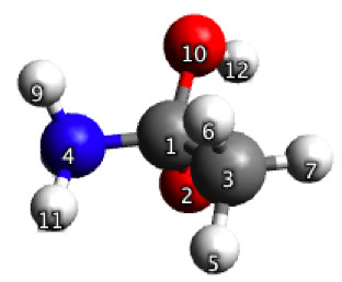
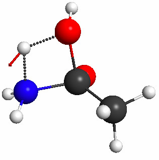
To start, I use Avogadro to build the geometry shown in Figure 5.32a and use it to construct the input file for an optimization with 4 constrained bond length.  The values for the constraints are taken from a paper.  Figure 5.32b shows the equilibrium geometry obtained with GAMESS, after 17 steps. Based on this geometry GAMESS finds the TS in three steps.


Figure 5.32a. Initial guess geometry for the constrained optimization discussed in Figure 5.33.
Click on the picture for an interactive version.
From Molecular Modeling Basics CRC Press, 2010


Figure 5.32b. The geometry resulting from the constrained optimization and the normal mode of the imaginary frequency computed for this structure at the PM3 level.
Click on the picture for an interactive version.
From Molecular Modeling Basics CRC Press, 2010

It will not always be possible to find an article that reports the TS structure for your reaction of interest. So let’s try to find the TS without the information from the article.  I start from the same structure (Figure 5.32a), and I arbitrarily pick C1-O10 as the reaction coordinate constrained to 1.70 Å.

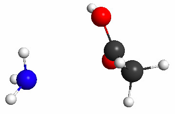
This constrained optimization results (after 23 steps) in the geometry shown in Figure 5.35a.  The subsequent TS search results in the geometry shown in Figure 5.35b, which has no imaginary frequency and is clearly the product.


Figure 5.35a. The geometry resulting from a constrained optimization in which the distance between atoms 1 and 10 (see Figure 5.32a for numbering) was constrained to 1.7 Å, and the normal mode of the imaginary frequency computed for this structure at the PM3 level.
Click on the picture for an interactive version.
From Molecular Modeling Basics CRC Press, 2010


Figure 5.35b. The geometry resulting from a TS search initiated from the geometry shown in Figure 5.35(a).
Click on the picture for an interactive version.
From Molecular Modeling Basics CRC Press, 2010

The fact that the C–O bond is re-formed indicates that it should be stretched more in the initial guess, so I repeat the optimization with the C–O distance constrained to 2.0 Å instead of 1.70 Å. This results (after 39 steps) in the geometry shown in Figure 5.36.  Using this as a starting geometry for the TS search leads to the TS in Figure 4.30a after 17 steps.


Figure 5.36. The geometry resulting from a constrained optimization in which the distance between atoms 1 and 10 (see Figure 5.32a for numbering) was constrained to 2.0 Å, and the normal mode of the imaginary frequency computed for this structure at the PM3 level.
Click on the picture for an interactive version.
From Molecular Modeling Basics CRC Press, 2010

In the screencast below I try to reproduce the calculations that lead to these figures.  Because I rebuild the structure in Figure 5.32a, I get different starting coordinates, so the energies and number of steps are different than what I discuss in the book for the 4-constraints approach.

In the case of the 1-constraint approach, I actually manage to find the TS using the 1.70 Å constraint.  Thus, the structures in Figures 5.35b and 5.36 do not appear in the screencast.  This just goes to show how finicky TS searchers are to starting geometries.


While editing the screencast I noticed that the PM3 energies of the two TS structures I find are very different (11 kcal/mol).  This is also true for the TSs I found when writing the book (where they are different by 6.6 kcal/mol).

This appears to be a problem that PM3 has with structures where bonds are partially broken or formed.  I could not reproduce this for structures with normal bond lengths such as the reactants and products.   Note that in the book, I use M06/6-31G(d) single point energies to compute barriers, and that the  M06/6-31G(d)//PM3 single point energies of the TSs found with the two different method are only different by 0.03 kcal/mol.